Floquet Formalism¶

Introduction¶

Many time-dependent problems of interest are periodic. The dynamics of such systems can be solved for directly by numerical integration of the Schrödinger or Master equation, using the time-dependent Hamiltonian. But they can also be transformed into time-independent problems using the Floquet formalism. Time-independent problems can be solve much more efficiently, so such a transformation is often very desirable.

In the standard derivations of the Lindblad and Bloch-Redfield master equations the Hamiltonian describing the system under consideration is assumed to be time independent. Thus, strictly speaking, the standard forms of these master equation formalisms should not blindly be applied to system with time-dependent Hamiltonians. However, in many relevant cases, in particular for weak driving, the standard master equations still turns out to be useful for many time-dependent problems. But a more rigorous approach would be to rederive the master equation taking the time-dependent nature of the Hamiltonian into account from the start. The Floquet-Markov Master equation is one such a formalism, with important applications for strongly driven systems (see e.g., [Gri98]).

Here we give an overview of how the Floquet and Floquet-Markov formalisms can be used for solving time-dependent problems in QuTiP. To introduce the terminology and naming conventions used in QuTiP we first give a brief summary of quantum Floquet theory.

Floquet theory for unitary evolution¶

The Schrödinger equation with a time-dependent Hamiltonian \(H(t)\) is

where \(\Psi(t)\) is the wave function solution. Here we are interested in problems with periodic time-dependence, i.e., the Hamiltonian satisfies \(H(t) = H(t+T)\) where \(T\) is the period. According to the Floquet theorem, there exist solutions to (1) on the form

where \(\Psi_\alpha(t)\) are the Floquet states (i.e., the set of wave function solutions to the Schrödinger equation), \(\Phi_\alpha(t)=\Phi_\alpha(t+T)\) are the periodic Floquet modes, and \(\epsilon_\alpha\) are the quasienergy levels. The quasienergy levels are constants in time, but only uniquely defined up to multiples of \(2\pi/T\) (i.e., unique value in the interval \([0, 2\pi/T]\)).

If we know the Floquet modes (for \(t \in [0,T]\)) and the quasienergies for a particular \(H(t)\), we can easily decompose any initial wavefunction \(\Psi(t=0)\) in the Floquet states and immediately obtain the solution for arbitrary \(t\)

where the coefficients \(c_\alpha\) are determined by the initial wavefunction \(\Psi(0) = \sum_\alpha c_\alpha \Psi_\alpha(0)\).

This formalism is useful for finding \(\Psi(t)\) for a given \(H(t)\) only if we can obtain the Floquet modes \(\Phi_a(t)\) and quasienergies \(\epsilon_\alpha\) more easily than directly solving (1). By substituting (2) into the Schrödinger equation (1) we obtain an eigenvalue equation for the Floquet modes and quasienergies

where \(\mathcal{H}(t) = H(t) - i\hbar\partial_t\). This eigenvalue problem could be solved analytically or numerically, but in QuTiP we use an alternative approach for numerically finding the Floquet states and quasienergies [see e.g. Creffield et al., Phys. Rev. B 67, 165301 (2003)]. Consider the propagator for the time-dependent Schrödinger equation (1), which by definition satisfies

Inserting the Floquet states from (2) into this expression results in

or, since \(\Phi_\alpha(T+t)=\Phi_\alpha(t)\),

which shows that the Floquet modes are eigenstates of the one-period propagator. We can therefore find the Floquet modes and quasienergies \(\epsilon_\alpha = -\hbar\arg(\eta_\alpha)/T\) by numerically calculating \(U(T+t,t)\) and diagonalizing it. In particular this method is useful to find \(\Phi_\alpha(0)\) by calculating and diagonalize \(U(T,0)\).

The Floquet modes at arbitrary time \(t\) can then be found by propagating \(\Phi_\alpha(0)\) to \(\Phi_\alpha(t)\) using the wave function propagator \(U(t,0)\Psi_\alpha(0) = \Psi_\alpha(t)\), which for the Floquet modes yields

so that \(\Phi_\alpha(t) = \exp(i\epsilon_\alpha t/\hbar) U(t,0)\Phi_\alpha(0)\). Since \(\Phi_\alpha(t)\) is periodic we only need to evaluate it for \(t \in [0, T]\), and from \(\Phi_\alpha(t \in [0,T])\) we can directly evaluate \(\Phi_\alpha(t)\), \(\Psi_\alpha(t)\) and \(\Psi(t)\) for arbitrary large \(t\).

Floquet formalism in QuTiP¶

QuTiP provides a family of functions to calculate the Floquet modes and quasi energies, Floquet state decomposition, etc., given a time-dependent Hamiltonian on the callback format, list-string format and list-callback format (see, e.g., qutip.mesolve for details).

Consider for example the case of a strongly driven two-level atom, described by the Hamiltonian

(5)¶\[ H(t) = -\frac{1}{2}\Delta\sigma_x - \frac{1}{2}\epsilon_0\sigma_z + \frac{1}{2}A\sin(\omega t)\sigma_z.\]

In QuTiP we can define this Hamiltonian as follows:

>>> delta = 0.2 * 2*np.pi
>>> eps0 = 1.0 * 2*np.pi
>>> A = 2.5 * 2*np.pi
>>> omega = 1.0 * 2*np.pi
>>> H0 = - delta/2.0 * sigmax() - eps0/2.0 * sigmaz()
>>> H1 = A/2.0 * sigmaz()
>>> args = {'w': omega}
>>> H = [H0, [H1, 'sin(w * t)']]

(png, hires.png, pdf)

The \(t=0\) Floquet modes corresponding to the Hamiltonian (5) can then be calculated using the qutip.floquet.floquet_modes function, which returns lists containing the Floquet modes and the quasienergies

>>> T = 2*np.pi / omega
>>> f_modes_0, f_energies = floquet_modes(H, T, args)
>>> f_energies 
array([-2.83131212,  2.83131212])
>>> f_modes_0 
[Quantum object: dims = [[2], [1]], shape = (2, 1), type = ket
Qobj data =
[[ 0.72964231+0.j      ]
 [-0.39993746+0.554682j]],
Quantum object: dims = [[2], [1]], shape = (2, 1), type = ket
Qobj data =
[[0.39993746+0.554682j]
 [0.72964231+0.j      ]]]

(png, hires.png, pdf)

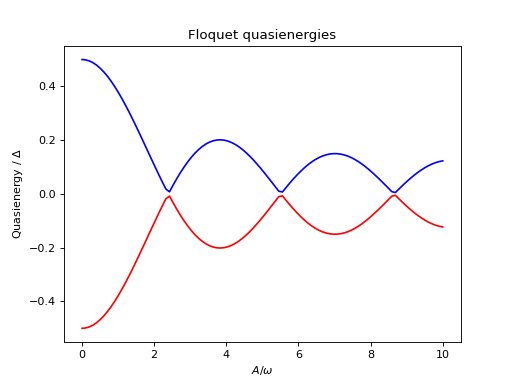
For some problems interesting observations can be draw from the quasienergy levels alone. Consider for example the quasienergies for the driven two-level system introduced above as a function of the driving amplitude, calculated and plotted in the following example. For certain driving amplitudes the quasienergy levels cross. Since the the quasienergies can be associated with the time-scale of the long-term dynamics due that the driving, degenerate quasienergies indicates a “freezing” of the dynamics (sometimes known as coherent destruction of tunneling).

>>> delta = 0.2 * 2*np.pi
>>> eps0  = 0.0 * 2*np.pi
>>> omega = 1.0 * 2*np.pi
>>> A_vec = np.linspace(0, 10, 100) * omega
>>> T = (2*np.pi)/omega
>>> tlist = np.linspace(0.0, 10 * T, 101)
>>> spsi0 = basis(2,0)
>>> q_energies = np.zeros((len(A_vec), 2))
>>> H0 = delta/2.0 * sigmaz() - eps0/2.0 * sigmax()
>>> args = {'w': omega}
>>> for idx, A in enumerate(A_vec): 
>>>   H1 = A/2.0 * sigmax() 
>>>   H = [H0, [H1, lambda t, args: np.sin(args['w']*t)]] 
>>>   f_modes, f_energies = floquet_modes(H, T, args, True) 
>>>   q_energies[idx,:] = f_energies 
>>> plt.figure() 
>>> plt.plot(A_vec/omega, q_energies[:,0] / delta, 'b', A_vec/omega, q_energies[:,1] / delta, 'r') 
>>> plt.xlabel(r'$A/\omega$') 
>>> plt.ylabel(r'Quasienergy / $\Delta$') 
>>> plt.title(r'Floquet quasienergies') 
>>> plt.show() 

(png, hires.png, pdf)¶

(png, hires.png, pdf)¶

Given the Floquet modes at \(t=0\), we obtain the Floquet mode at some later time \(t\) using the function qutip.floquet.floquet_mode_t:

>>> f_modes_t = floquet_modes_t(f_modes_0, f_energies, 2.5, H, T, args)
>>> f_modes_t 
[Quantum object: dims = [[2], [1]], shape = (2, 1), type = ket
Qobj data =
[[-0.89630512-0.23191946j]
 [ 0.37793106-0.00431336j]],
Quantum object: dims = [[2], [1]], shape = (2, 1), type = ket
Qobj data =
[[-0.37793106-0.00431336j]
 [-0.89630512+0.23191946j]]]

The purpose of calculating the Floquet modes is to find the wavefunction solution to the original problem (5) given some initial state \(\left|\psi_0\right>\). To do that, we first need to decompose the initial state in the Floquet states, using the function qutip.floquet.floquet_state_decomposition

>>> psi0 = rand_ket(2)
>>> f_coeff = floquet_state_decomposition(f_modes_0, f_energies, psi0)
>>> f_coeff 
[(-0.645265993068382+0.7304552549315746j),
(0.15517002114250228-0.1612116102238258j)]

and given this decomposition of the initial state in the Floquet states we can easily evaluate the wavefunction that is the solution to (5) at an arbitrary time \(t\) using the function qutip.floquet.floquet_wavefunction_t

>>> t = 10 * np.random.rand()
>>> psi_t = floquet_wavefunction_t(f_modes_0, f_energies, f_coeff, t, H, T, args)

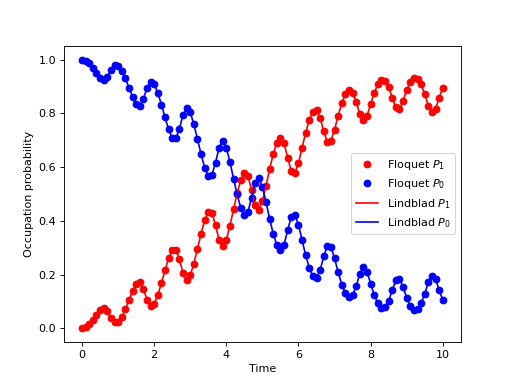
The following example illustrates how to use the functions introduced above to calculate and plot the time-evolution of (5).

import numpy as np
from matplotlib import pyplot

import qutip

delta = 0.2 * 2*np.pi
eps0  = 1.0 * 2*np.pi
A     = 0.5 * 2*np.pi
omega = 1.0 * 2*np.pi
T      = (2*np.pi)/omega
tlist  = np.linspace(0.0, 10 * T, 101)
psi0   = qutip.basis(2, 0)

H0 = - delta/2.0 * qutip.sigmax() - eps0/2.0 * qutip.sigmaz()
H1 = A/2.0 * qutip.sigmaz()
args = {'w': omega}
H = [H0, [H1, lambda t,args: np.sin(args['w'] * t)]]

# find the floquet modes for the time-dependent hamiltonian
f_modes_0,f_energies = qutip.floquet_modes(H, T, args)

# decompose the inital state in the floquet modes
f_coeff = qutip.floquet_state_decomposition(f_modes_0, f_energies, psi0)

# calculate the wavefunctions using the from the floquet modes
p_ex = np.zeros(len(tlist))
for n, t in enumerate(tlist):
    psi_t = qutip.floquet_wavefunction_t(f_modes_0, f_energies, f_coeff, t, H, T, args)
    p_ex[n] = qutip.expect(qutip.num(2), psi_t)

# For reference: calculate the same thing with mesolve
p_ex_ref = qutip.mesolve(H, psi0, tlist, [], [qutip.num(2)], args).expect[0]

# plot the results
pyplot.plot(tlist, np.real(p_ex),     'ro', tlist, 1-np.real(p_ex),     'bo')
pyplot.plot(tlist, np.real(p_ex_ref), 'r',  tlist, 1-np.real(p_ex_ref), 'b')
pyplot.xlabel('Time')
pyplot.ylabel('Occupation probability')
pyplot.legend(("Floquet $P_1$", "Floquet $P_0$", "Lindblad $P_1$", "Lindblad $P_0$"))
pyplot.show()

(png, hires.png, pdf)

Pre-computing the Floquet modes for one period¶

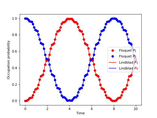
When evaluating the Floquet states or the wavefunction at many points in time it is useful to pre-compute the Floquet modes for the first period of the driving with the required resolution. In QuTiP the function qutip.floquet.floquet_modes_table calculates a table of Floquet modes which later can be used together with the function qutip.floquet.floquet_modes_t_lookup to efficiently lookup the Floquet mode at an arbitrary time. The following example illustrates how the example from the previous section can be solved more efficiently using these functions for pre-computing the Floquet modes.

import numpy as np
from matplotlib import pyplot
import qutip

delta = 0.0  * 2*np.pi
eps0  = 1.0 * 2*np.pi
A     = 0.25 * 2*np.pi
omega = 1.0 * 2*np.pi
T      = 2*np.pi / omega
tlist  = np.linspace(0.0, 10 * T, 101)
psi0   = qutip.basis(2,0)

H0 = - delta/2.0 * qutip.sigmax() - eps0/2.0 * qutip.sigmaz()
H1 = A/2.0 * qutip.sigmax()
args = {'w': omega}
H = [H0, [H1, lambda t, args: np.sin(args['w'] * t)]]

# find the floquet modes for the time-dependent hamiltonian        
f_modes_0,f_energies = qutip.floquet_modes(H, T, args)

# decompose the inital state in the floquet modes
f_coeff = qutip.floquet_state_decomposition(f_modes_0, f_energies, psi0)

# calculate the wavefunctions using the from the floquet modes
f_modes_table_t = qutip.floquet_modes_table(f_modes_0, f_energies, tlist, H, T, args)
p_ex = np.zeros(len(tlist))
for n, t in enumerate(tlist):
    f_modes_t = qutip.floquet_modes_t_lookup(f_modes_table_t, t, T)
    psi_t     = qutip.floquet_wavefunction(f_modes_t, f_energies, f_coeff, t)
    p_ex[n] = qutip.expect(qutip.num(2), psi_t)

# For reference: calculate the same thing with mesolve
p_ex_ref = qutip.mesolve(H, psi0, tlist, [], [qutip.num(2)], args).expect[0]

# plot the results
pyplot.plot(tlist, np.real(p_ex),     'ro', tlist, 1-np.real(p_ex),     'bo')
pyplot.plot(tlist, np.real(p_ex_ref), 'r',  tlist, 1-np.real(p_ex_ref), 'b')
pyplot.xlabel('Time')
pyplot.ylabel('Occupation probability')
pyplot.legend(("Floquet $P_1$", "Floquet $P_0$", "Lindblad $P_1$", "Lindblad $P_0$"))
pyplot.show()

(png, hires.png, pdf)

Note that the parameters and the Hamiltonian used in this example is not the same as in the previous section, and hence the different appearance of the resulting figure.

For convenience, all the steps described above for calculating the evolution of a quantum system using the Floquet formalisms are encapsulated in the function qutip.floquet.fsesolve. Using this function, we could have achieved the same results as in the examples above using

output = fsesolve(H, psi0, times, [num(2)], args)
p_ex = output.expect[0]

Floquet theory for dissipative evolution¶

A driven system that is interacting with its environment is not necessarily well described by the standard Lindblad master equation, since its dissipation process could be time-dependent due to the driving. In such cases a rigorious approach would be to take the driving into account when deriving the master equation. This can be done in many different ways, but one way common approach is to derive the master equation in the Floquet basis. That approach results in the so-called Floquet-Markov master equation, see Grifoni et al., Physics Reports 304, 299 (1998) for details.

The Floquet-Markov master equation in QuTiP¶

The QuTiP function qutip.floquet.fmmesolve implements the Floquet-Markov master equation. It calculates the dynamics of a system given its initial state, a time-dependent hamiltonian, a list of operators through which the system couples to its environment and a list of corresponding spectral-density functions that describes the environment. In contrast to the qutip.mesolve and qutip.mcsolve, and the qutip.floquet.fmmesolve does characterize the environment with dissipation rates, but extract the strength of the coupling to the environment from the noise spectral-density functions and the instantaneous Hamiltonian parameters (similar to the Bloch-Redfield master equation solver qutip.bloch_redfield.brmesolve).

Note

Currently the qutip.floquet.fmmesolve can only accept a single environment coupling operator and spectral-density function.

The noise spectral-density function of the environment is implemented as a Python callback function that is passed to the solver. For example:

gamma1 = 0.1
def noise_spectrum(omega):
    return 0.5 * gamma1 * omega/(2*pi)

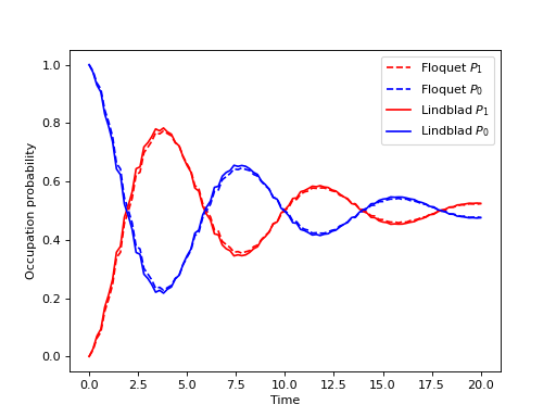
The other parameters are similar to the qutip.mesolve and qutip.mcsolve, and the same format for the return value is used qutip.solver.Result. The following example extends the example studied above, and uses qutip.floquet.fmmesolve to introduce dissipation into the calculation

import numpy as np
from matplotlib import pyplot
import qutip

delta = 0.0  * 2*np.pi
eps0  = 1.0 * 2*np.pi
A     = 0.25 * 2*np.pi
omega = 1.0 * 2*np.pi
T      = 2*np.pi / omega
tlist  = np.linspace(0.0, 20 * T, 101)
psi0   = qutip.basis(2,0)

H0 = - delta/2.0 * qutip.sigmax() - eps0/2.0 * qutip.sigmaz()
H1 = A/2.0 * qutip.sigmax()
args = {'w': omega}
H = [H0, [H1, lambda t,args: np.sin(args['w'] * t)]]

# noise power spectrum
gamma1 = 0.1
def noise_spectrum(omega):
    return 0.5 * gamma1 * omega/(2*np.pi)

# find the floquet modes for the time-dependent hamiltonian        
f_modes_0, f_energies = qutip.floquet_modes(H, T, args)

# precalculate mode table
f_modes_table_t = qutip.floquet_modes_table(
    f_modes_0, f_energies, np.linspace(0, T, 500 + 1), H, T, args,
)

# solve the floquet-markov master equation
output = qutip.fmmesolve(H, psi0, tlist, [qutip.sigmax()], [], [noise_spectrum], T, args)

# calculate expectation values in the computational basis
p_ex = np.zeros(tlist.shape, dtype=np.complex128)
for idx, t in enumerate(tlist):
    f_modes_t = qutip.floquet_modes_t_lookup(f_modes_table_t, t, T)
    p_ex[idx] = qutip.expect(qutip.num(2), output.states[idx].transform(f_modes_t, True))

# For reference: calculate the same thing with mesolve
output = qutip.mesolve(H, psi0, tlist,
                       [np.sqrt(gamma1) * qutip.sigmax()], [qutip.num(2)],
                       args)
p_ex_ref = output.expect[0]

# plot the results
pyplot.plot(tlist, np.real(p_ex), 'r--', tlist, 1-np.real(p_ex), 'b--')
pyplot.plot(tlist, np.real(p_ex_ref), 'r', tlist, 1-np.real(p_ex_ref), 'b')
pyplot.xlabel('Time')
pyplot.ylabel('Occupation probability')
pyplot.legend(("Floquet $P_1$", "Floquet $P_0$", "Lindblad $P_1$", "Lindblad $P_0$"))
pyplot.show()

(png, hires.png, pdf)

Alternatively, we can let the qutip.floquet.fmmesolve function transform the density matrix at each time step back to the computational basis, and calculating the expectation values for us, but using:

output = fmmesolve(H, psi0, tlist, [sigmax()], [num(2)], [noise_spectrum], T, args)
p_ex = output.expect[0]